Abstract
A brief overview of utility functions, their uses, properties and some examples.
Utility
Utility is used to model total satisfaction or benefit gained from having a certain wealth, consuming a good or consuming a service. Theories based off the idea of a rational consumer usually assume that people will try and maximise their utility, that is, maximise their total satisfaction. It is often used to evaluate situations without an immediate pay back and uncertainty in the outcome.
Utility directly influences demand, as the higher the utility of a product or service the more consumers will want it. As a consequence, utility also influences the price of a good or service.
Utility Functions
Assume there is some set of possible alternatives, , from which an agent can either choose an alternative, or be assigned an alternative based off some probability distribution (situation dependent).
The set has a binary relation, , that allows any two elements of the set to be compared. This binary relation models the agents preference, with the agent preferring to if . Put differently, if then alternative brings the agent more satisfaction.
It is also assumed that possible alternatives can be mixed according to some probability distribution, with the mixture being a valid alternative, such that for two elements ,
A utility function, , is a map from the set to the real numbers that preserves the ordering enforced by the binary relation. Hence, , such that
Formally, this means that utility functions are a monotone for the binary relation.
A utility function subject to a linear transformation will continue to be monotonic for the binary relation on . Hence, the numerical output of a utility function does not hold any intrinsic value. It is comparisons between the utility of different alternatives that has meaning.
Utility functions allow the idea of risk to be introduced for agents. Typically, they will include an additional parameter that is used to model the agents attitude toward risk. This will be denoted by .
Utility Axioms
Let be a set of alternative outcomes.
There exists a binary relation on , namely , and an operations that allows alternative outcomes to be combined via some probability distribution to form new alternative outcomes,
If these axioms are satisfied then there exists a function that preserve the ordering set on by the binary relation.
forms a total ordering on .
This means that for all pairs of elements, one of the following relations is true
and if and then 💭.
Physical Interpretation: The agent has a preference over all possible alternatives. There is no set of possible alternative where they are “not sure” which alternative they prefer.
implies
Physical Interpretation: If is preferable to then having any probability of obtaining the alternative is preferable to having with certainty.
implies
Physical Interpretation: If is preferable to then having any probability of obtaining the alternative is less-preferable to having with certainty. This is the alternative case to 2.
implies the existence of an such that
Physical Interpretation: Regardless of how preferable is compared to , there exists a probability of occurring that is small enough compared to the probability of the less preferable alternative occurring such that taking the chance is less preferable then taking with certainty.
implies the existence of an such that
Physical Interpretation: Regardless of how less preferable is compared to , there exists a probability of occurring that is small enough compared to the probability of the more preferable alternative occurring such that taking the chance is more preferable then taking with certainty.
These axioms were taken from Theory of Games and Economic Behavior
Expected Utility
In general, one assumes that there is some probability distribution of the potential alternatives, with the alternative occuring with probability such that
From this probability distribution, one can consider the expected alternative as
This is the average alterative the agent would get if they sampled from the alternatives according to the probability distribution over them 💭.
The utility of this expected alternative if then given by .
The utility of each outcome is also described by some probability distribution where the agent has utility with probability . This means that the expected utility can be found from
A rational agent will aim to maxamise their expected utility, i.e, maxamise their satisfaction.
Certainty Equivalent
The certainty equivalent, , is the alternative that the agent is as satisfied with as the expected alternative,
where is the how satisfied the agent is with the alternative .
The certainty equivalent is therefore the alternative such that the utility of that alternative would give the agent the average utility over all alternatives. Hence, if the agent had the alternative this would return them the expected amount of satisfaction (the expected utility)
Risk from Utility
Consider that there is a probability distribution over all alternatives, with probability of getting an outcome . All the alternatives are totalled ordered due to preference, therefore, if taking a alternative from the distribution, there is some probability of the agent getting a high ranked preference, and some probability of the agent getting a low ranked preference.
Assume that an agent is given the choice to either take an alterative from the distribution or they take the alterative given by the certainty equivalent, , with certainty .
How the certainty equivalent, , relates to the expected alternative, , tells us about the risk profile of the agent.
If the agent is risk adverse.
The agent is cautious, they are happy to accept a definite alterative that is less preferable then the alternative they are expecting to get from the distribution. They do this to avoid the possibility of getting an even less preferable alternative from the distribution.
If the agent is risk neutral.
The agent will choose whichever option will give them the most preferable alternative.
If the agent is risk seeking.
The agent is not cautious, they will only take the definite alternative if it is more preferable then the alternative they are expect to get from the distribution. This is because they are happy to take the possibility of getting a less preferable alternative in the hope of getting a more preferable alternative.
These risk profiles are encoded into the curvature of the utility functions.
Example Utility Functions
Let be some variable of importance to an agent and a parameter that models risk.
An example of an isoelastic utility function is
Let be some variable of importance to an agent and a parameter that models risk.
An example of an exponential utility function is
is the degree of risk preference
and the agent is risk-averse.
and the agent is risk-neutral.
and the agent is risk-seeking.
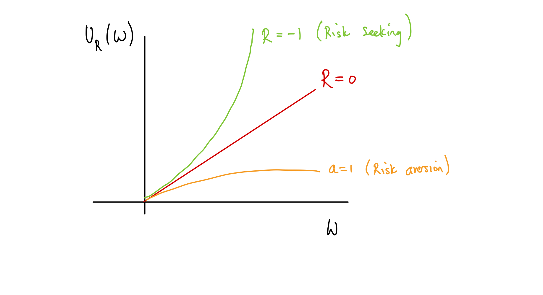
How the exponential utility functions changes with varying risk parameter, .