Abstract
The stabilizer formalism of quantum error correction.
The stabilizer formalism is a method for creating error correcting codes using the Pauli-group. In addition to allowing certain errors to be detected and correct, logical gates can also be performed in this framework.
Pauli-group
The generators of the qubit Pauli-group are
From these operators all elements of the one qubit Pauli-group can be generated. The Pauli-group is the set of Pauli-operators plus identity with all possible phases of .
The -qubit Pauli-group , , is then the -fold tensor product of elements in the one qubit Pauli-group. All elements in either commute or anit-commute,
All elements of the Pauli-group have eigenvalues or . Here, we mostly consider just the elements with eigenvalues (the Hermitian elements of the Pauli-group).
Stabilizer Codes
Definition
The stabilizers of an error correcting code are defined as
such that . The stabilizers are therefore an Abelian subgroup of the -qubit Pauli-group, , such that all logical states (states in the code space) are eigenstates of each stabilizer, that does not contain the negative identity operator.
The justification of these conditions are as follows:
:
This avoids any logical information encoded in the code space being destroyed when a stablizer is measured on .
Further Details
A state, is said to be stabilized by an operator if , meaning is a eigenstate of .
From the above definition of , it can be seen that all logical states are stabilized by . Therefore, if one were to measure or apply on any logical state they would return the state unchanged. This avoids any logical information encoded in the code space being destroyed when a stablizer is measured on . (Does it also prevent loss of logical information in general? I am currently not sure).
One can reverse this definition, and defined the code space to be the subspace of the total Hilbert space that is stabilized by all elements of . Phrased alternatively, the code space is defined as the intersection of all eigenspaces of the elements of .
:
If this condition is not met, only the trivial space can be stabilized.
Proof
Let such that . Moreover, assume they both stabilize such that
Firstly, note that given that all elements of commute or anti-commute,
Secondly, the products, and also stabilize if and individually stabilize , such that
Putting these facts together implies that
This is only true if , meaning that non-Abelian subgroups of can only stabilize a trivial subspace.
(Note, the equation is about the physical equivalence of vectors in a Hilbert space, with this equation only being satasfied for the zero vector. It is not about whether two states are physically distinguishable under global phases.)
:
If this condition is not met, only the trivial space can be stabilized.
Operation
A stablizer code works by first encoding a logical state into a subspace. Each stablizer in the set is then measured, with each measurement giving an output of +1 or -1. From these measurement outcomes one can establish if an error from a given set has occurred and offer a method to correct it.
We will work through the logic of these codes step by step.
Preliminaries
We will first build an error correcting code able to correct a single error.
An error correcting code is defined by first establishing a set of code words. These are typically a set of orthogonal pure states such that . The code space, , is then the subspace of the full Hilbert space, , spanned by the set of code words,
The logical state is then some state encoded within this code space, . We define to be the projector onto the code space,
If some unitary error, , acts on the logical state, the state will be mapped to the space spanned by acting on the code words,
where we define this subspace and the projector onto the space as
The goal of the simplest imaginable error correcting code is then to (a) determine which of or has been applied to the logical state without (b) disturbing the logical state and hence destroying the encoded information.
Criteria (a) can be considered as an example of quantum channel discrimination, where the logical state is the reference state, with the added constraint of criteria (b).
Error Correction as Quantum Channel Discrimination
In the task of quantum channel discrimination one considers two parties, Alice and a referee. The referee has some reference state, , and a predetermined set of quantum channels . Both the reference state and the set of quantum channels are known to Alice.
The referee chooses an index and then applies the channel to the reference state. The referee then sends the state to Alice. Alice makes a measurement on the state with the intention of identify the channel the referee applied. The ultimate output of the measurement will therefore be some index , such that if Alice has succeed in the task and if she has failed.
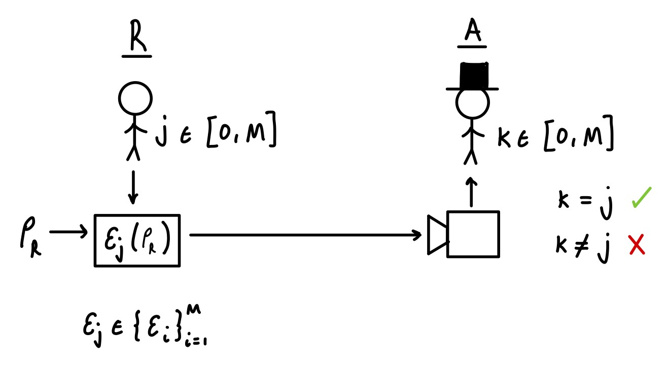
A schematic of a quantum channel discrimination task. R and A are the referee and Alice respectively. The referee applies a channel from a predetermined set to the reference state and then sends it to Alice. Alice performs a measurement on the state and aims to identify which channel the referee applied.
With some added constraints, error correction can be reframed as a quantum channel discrimination task. The reference state is no-longer a predetermined state but rather an arbitrary state within some predetermined subspace. The referee is then the noise, with it being assumed that the noise is restricted to some likely set of possible channels. Finally, Alice is the decoder of the error correction protocol aiming to identify which error has occurred.
The major addition to quantum error correction is the need for the logical information encoded into the subspace to not be disturbed by the measurement made by Alice (the decoder). Practically, this means a restriction on the measurements Alice is allowed to perform.
It is a well known result in quantum information theory that for two quantum states to be deterministically distinguishable they must be orthogonal. Here, we are not concerned with specific states, but rather arbitary states encoded into subspaces. However, the result instead just applies to the subspaces. Hence, it is only possible to deterministically determine if or has been applied to the logical state if
meaning that for any arbitrary state , it is the case that .
If this first condition is met it is always the case that one can find a projector , such that
where is the projector onto the reminder of the Hilbert space not covered by and . This will defined a subspace orthogonal to both and and is simply given by . From here, one can then defined an observable
that can be seen to fulfil both criteria (a) and (b). It fulfils (a) as if has been applied (no error) then
meaning one gets the outcome with certainty. If instead has been applied then
meaning one gets the outcome with certainty. The observable therefore allows one to determine which error has occurred with certainty. It fulfils (b) as the
meaning the states remain unchanged after the measurements.
The error correcting code can be summarised as follows: if the errors that can occur are and the code space is , then measure the observable and if the outcome is do nothing, if it is apply .
The logic above can be easily expanded to multiple errors. Assume the set of possible errors is , where . Each error must then map an arbitrary state to an orthogonal subspace such that
Correctable Errors
The Role of the Stabilizers
Given the set of stabilizers is defined for an arbitrary state within the code space, the set of stablizers should be thought of as stabilizing the code space rather than a given logical state. In reality, the code space is defined in the opposite direction: each stabliser, , is an element of the Pauli-group and can hence be written as
where is the projector onto the +1 eigenspace , and the projector onto the -1 eigenspace. One can then defined the code space, via the projector on the space , as
Measuring Stabilizer
All elements of are unitary. If is also Hermitian, then any stabilizer can be measured on the logic state indirectly, with the measurement outcome stored in an ancilla 💭.
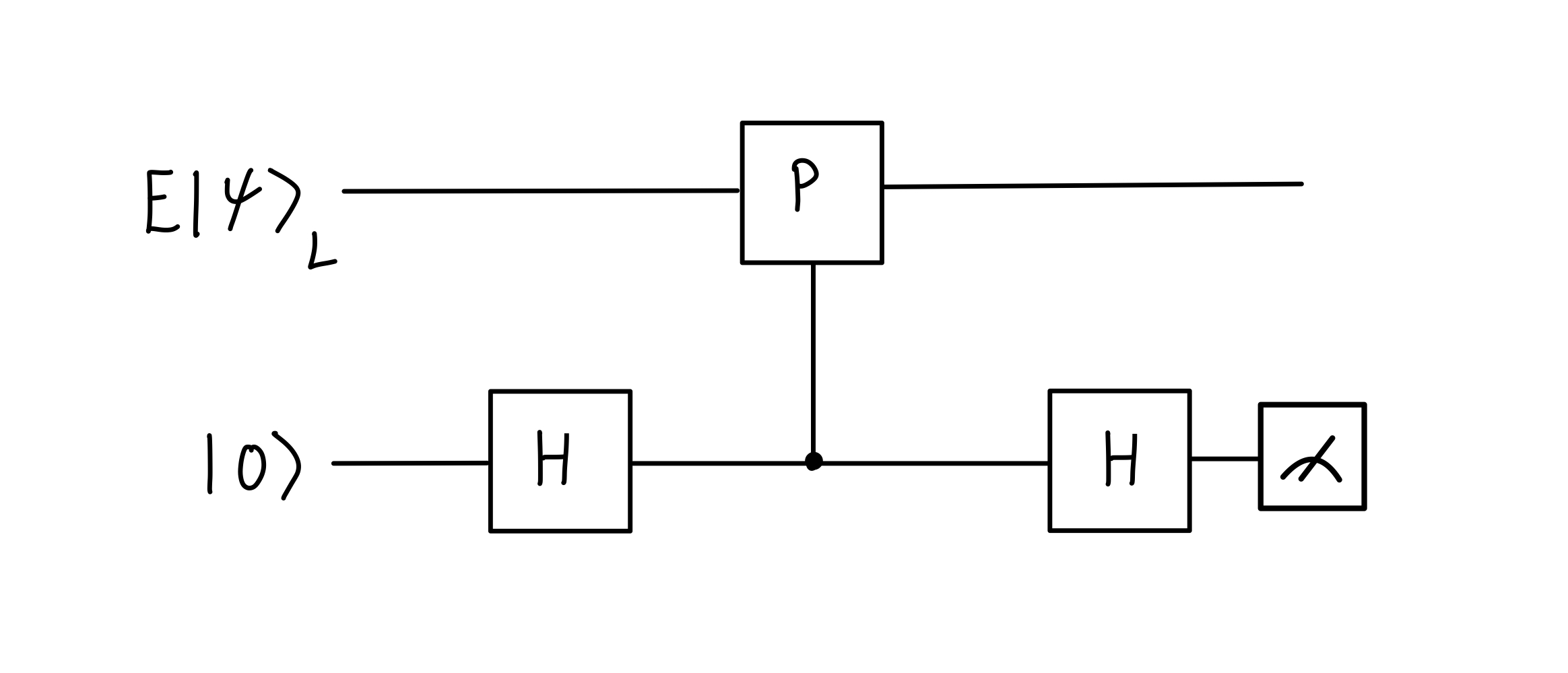
A schematic of the circuit used to measure the stabilizer on the logical state .
Assume that is a stabilizer of the logical state such that . Let be some correctable error that has occurred on the logical state, such that or , depending on whether is in the positive or negative eigenspace of .
The input state into the circuit is , where labels the ancillary space and the subscript now doubles as a label for the space of the logical state.
The output state is then
Proof
Therefore, if , the second term will go to zero and the output state becomes
such that if one measures on the ancilla they will get the outcome +1 (syndrome bit 0) with certainty.
If , the first term will go to zero and the output state becomes
such that a measurement performed on the ancilla now gives the outcome -1 (syndrome bit 1) with certainty.
By performing the above circuit and measuring the ancilla one can therefore determine if the logical state is in the +1 or -1 eigenspace of the stabilizer .
Note, this method of performing measurements only really works for measuring observables in on stabilizer states.
Parity Measurements Circuits
When discussing the 2-bit repetition code it was noted that the measurement of the stabilizer was akin to performing a parity check on the qubits. Specifically, a logical qubit was encoded into space such that
It was then seen that it was possible to perform error detection on the set of errors by measuring the stabilizer . If occurs, the state stays in the code space and measuring the stabilizer gives the output +1 (syndrome bit 0). If either an or occurs, the state is mapped into the space , and a measurement of the stabilizer gives the output -1 (syndrome bit 1).
A simpler circuit can be used for measuring stabilizers that perform a parity check. The circuit for performing the parity check in the 2-bit repetition code is shown in the below figure.
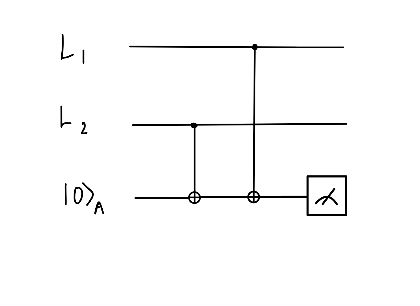
A circuit that checks the parity of two qubits and stores the result in an ancilla. and are used to label the two physical qubits used to create the single logical qubit.
Firstly, the parity of two bits, , is given by . This will be zero if both bits are zero or both bits are one. If the bits differ, it will be one.
Now, note that the action of a CNOT gate on some arbitrary computational basis state can be written as
This works because a CNOT gate applies an gate to the second qubit if the first qubit is . This gate will flip the second qubit, which can be done by adding 1 to it. Hence, if nothing is added to the second qubit and it remains . If then 1 is added to , flipping it.
From here, consider that if it is not known if an error has occurred on an arbitrary qubit encoded into the code space, , the state can be written as
The input into the circuit is then
The action of the first CNOT gate is then
as . The action of the second CNOT gate is then
as . Hence, if is measured on the computational basis then the parity is output with certainty.