Abstract
Some details about classical and quantum entropy functions
Broadly, entropy functions describe the level of uncertainty in a probability distribution. Here, we detail the underlying concepts that leads to the construction of entropy functions.
Information gain or Surprisal
Consider a discrete random variable , where the one gets the outcome with probability . If there are possible outcomes, this can be described by the probability distribution
If one looks at the outcome of the random variable and sees that it is , then the information they have gained from now knowing this is defined by
It can be seen that if the outcome occurs with high probability, then is very small; if the outcome occurs with low probability, then is very large. That is, we gain lots of information if we are surprised about the outcome i.e., that event had a low probability of occurring. For this reason, the function is sometimes refereed to as the surprisal.
Mathematical Justifications for
The mathematical justifications for being the correct function for quantify the information gain is:
The information gain should depend only on the probability of a given outcome occurring, not on its label.
Given a probability distribution it should not matter if this gives the outcomes of a coin or the color of ball, the theory of the information gain should be independent of the physical system in which that information is encoded.
The function should be a smooth function of probability.
This means there are no jumps in the function and it varies continuously from max information gain to minimum information gain.
The probability of two independent events and occurring is . This condition then means that the information gained from the two independent events occurring is the sum of the information gained from the individual events. This can be justified physically, as if the events are independent then learning about one should not tell us about the other.
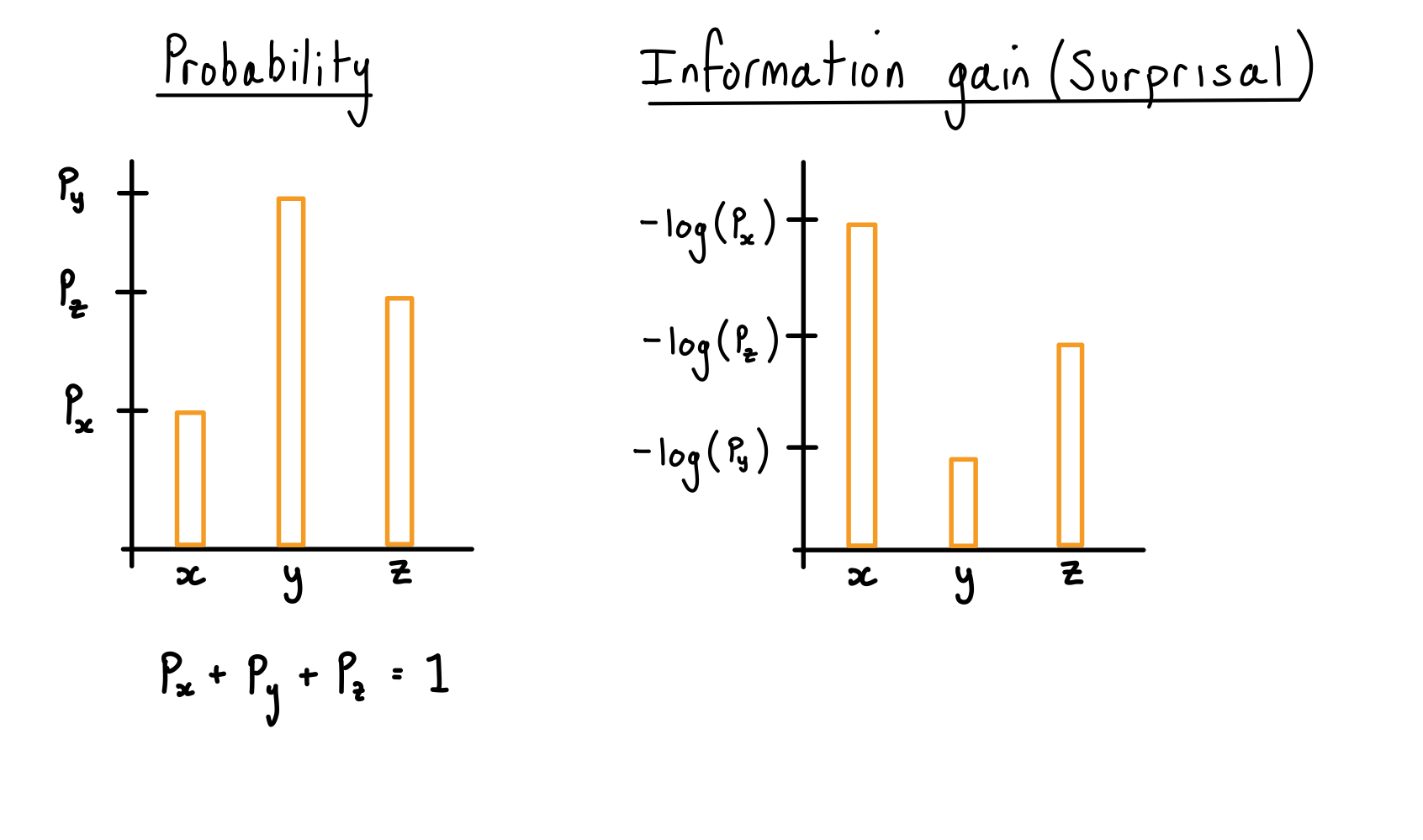
The probability distribution of getting each outcome of a random variable as compared to the information gain of getting each outcome (the surprisal).
Entropies
The Shannon entropy of the random variable is then nothing more then the average information gain:
where is the expectation value of over the probability distribution .
The entropy can be thought of as either:
a measure of the uncertainty in the outcome of the random variable before the outcome is known
a measure of how much information is gained after the outcome of a random variable becomes known.
Example
Let the random variable have a probability distribution
The information gain or surprisal is then
where we have chosen to use log based two.
The entropy is then
We now compare this to the extreme distributions
which are the certain and maximally uncertain distributions respectively. These then have entropy
Given , there is no uncertainty in the outcome of the random variable, we therefore learn nothing when the outcome becomes known, and the entropy is zero.
Given , there is maximum uncertainty in the outcome of the random variable, we therefore gain the maximum amount of information when the outcome becomes known, and the entropy is maximum.
It can then be seen that, given , we have
meaning that the uncertainty before the outcome of the random variable becomes know, or the information gained after, sits between these two extreme distributions.
Through the noiseless coding theorem, the entropy has an operational interpretation, which gives it a solid grounding in practical reality: given a two outcome random variable with , from which outputs have been collected, bits are needed to stored these outputs.
Generalised Entropies
Given a set of numbers that are distributed via some probability distribution, the mean is not the only function that can be used to aggregate the set of numbers.
Specifically, one can generalise the notion of means using Kolmogorov–Nagumo averages.
Let be a set of different numbers, and let be a continuous and injective (one-to-one) function.
The mean of is
If for some constants and , this reduces to the arithmetic mean.
Using the Kolmogorov–Nagumo averages, a general entropy function can then be defined as
where each element is weighted by its probability of occurring, rather then equally as in the definition of the Kolmogorov–Nagumo averages given above.
Using this, it can be seen that the Shannon entropy is a special case of the mean of the information gain of a probability distribution where .
-Rényi Entropies
Rényi looked for functions that made additive for two independent random variables, as this was a desirable feature of the Shannon entropy. In addition to , it was found also made additive, where is a parameter and a constant.
Using this for gives the so-called -Rényi Entropies:
For it is defined via the limits towards these values.
Just as different means inform us about different features of a set of numbers, the different Rényi entropies informs us about different features of the information gain of a distribution.
It can be shown that
meaning that in the limit of tending toward one, the Rényi entropy becomes the Shannon entropy.