Abstract
Details of the task of quantum state Teleportation, in both the qubit and higher dimensional case. The fidelity of teleportation and teleportation from the perspective of the resource theory of entanglement is also discussed.
Setup
Let there be two spatially separated parties, Alice (A) and Bob (B), who share a dimension maximally entangled bipartite state,
It is assumed they have the ability to perform any operation on a quantum system in their respective labs and that they can send any amount of classical information to each other 💭.
These operations are known as the set of local operations and classical communication () 💭. They are a physically motivated set of operations as local manipulation of quantum states and classical communication between spatially separated parties are much easier to perform then the transportation of quantum states between spatially separated parties.
Alice has a single copy of the qubit,
in her laboratory that she wants to send to Bob. The subscript shows that the state is in Alice’s lab. Given Alice and Bob can only send classical information to each other, Alice cannot send the qubit to Bob directly.
Teleportation Protocol
Alice can instead send the qubit to Bob via the quantum teleportation protocol.
The quantum teleportation protocol states that it is possible for Alice to exactly send the state to Bob using: a maximally entangled state, a measurement in a maximally entangled basis, two classical bits and one local unitary.
The Protocol:
The initial state shared between Alice and Bob is
This state, , can then be expanded and rewritten as
Firstly, Alice measures the operator, , which has the Bell states as its eigenvectors,
where , and
on the spaces . Alice gets one the eigenvalues of as her measurement outcome.
After Alice measures , the state of Bob’s system is dependent on Alice’s measurement outcome:
Therefore, based on her measurement outcome Alice knows which state Bob has in his system. Bob, however, does not know which of the above states he has in his system.
Secondly, Alice communicates her measurement outcome to Bob, therefore informing him of the state of his system. Given there were four possible outcomes, , she needs to send Bob two bits ():
After receiving the two bits from Alice, Bob knows which of four states he has (but not and explicitly.)
Lastly, and conditioned on the bits he receives from Alice, Bob applies one of four unitaries:
After this, Bob is left with the state in his space.
Hence, using one maximally entangled state, one measurement in the Bell basis, two classical bits and one local unitary, the state has been “sent” from Alice to Bob. However, the physical state has not been sent, the information that defines the state has been.
Diagram
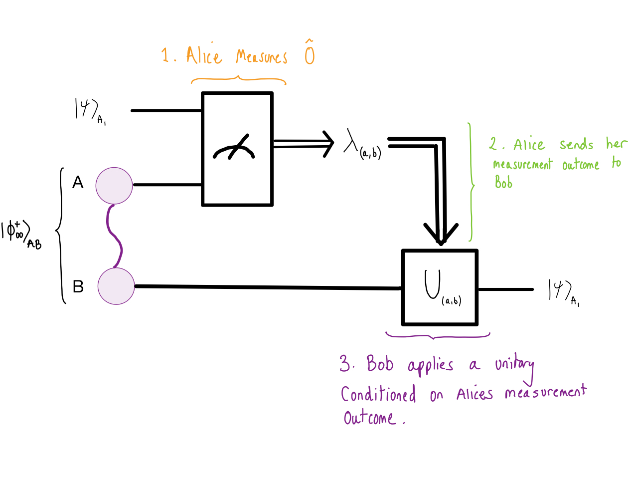
A graphical depiction of the quantum teleportation protocol.
Fidelity of Teleportation
One does not need a maximally entangled state to perform teleportation. However, using a partially entangled state - a state that is entangled but not maximally entangled - will reduce the quality of the teleportation, as measured by the fidelity of teleportation. This is a measure of how similar the final quantum state in Bob’s space is to the initial state Alice is trying to teleport.
Details
The average fidelity of teleportation is given by
where is a shared state between Alice and Bob, is the state being teleported, where , and is the teleportation channel (this packages up the measurement of , the classical communication and the local rotation). The fidelity is a measure of how well a state performs on average at teleporting all possible states in the space from Alice to Bob.
Properties
iif is the maximally entangled state.
If is a separable state, then there exists a classical strategy such that .
The fidelity of teleportation has been related to the entanglement fraction as
where
The entanglement fraction maximises the overlap between the state and the maximally entangled state over all protocols.
Higher Dimensional Systems
The teleportation protocol can be generalised to send higher dimensional states between two spatially separated parties. A state , where , can be teleported between Alice (A) and Bob (B) using a bipartie maximally entangled state of local dimension ,
Firstly, Alice measures the operator with a basis of maximally entangled states,
where are the so called Heisenberg-Weyl operators. See generating a maximally entangled basis for more details on this.
Secondly, Alice needs to send the results of her measurement outcome, which can be capture by pair of values , to Bob. There are different pairs of values , meaning Alice needs to send bits to Bob.
Lastly, if Bob receives the bits from Alice associated to a pair of values , Bob applied to his local system. Bob then has the dimensional state in his system.
Teleportation in the Resource Theory of Entanglement
In the teleportation protocol, after Alice measures , Alice and Bob no longer share a maximally entangled state; the maximally entangled state has been “consumed” in order to implement the teleportation protocol. Given one cannot perform teleportation without an entangled state and it is consumed in the process it is considered a resource for the task.
The teleportation protocol is an example of simulating a channel in a resource theory. Specifically, the teleportation channel allows the simulation of a noiseless quantum channel in the resource theory of entanglement.
Details
The allowed operations of the resource theory of entanglement are - local operations and classical communication between two spatially separated parties Alice () and Bob (). The free states are the set of all product states, as any product state between Alice and Bob can be generated via and, given any product state between and , no entanglement can be generated via .
There is no channel in the set of allowed operations to send a quantum state from Alice to Bob. However, when the two parties share an entangled state - a maximally resourceful state - there exists an allowed operation, that is an channel, that is able to simulate a noiseless quantum channel that sends a quantum state from Alice to Bob. Formally,
where is the quantum channel for the teleportation protocol and is the quantum channel that noiselessly sends the quantum state from Alice to Bob.
As measured by the fidelity of teleportation, Alice and Bob can perform lower quality teleportation if is entangled but not maximally entangled. In this case, the channel that is simulated is not noiseless, but instead noisy. Bob’s final state will therefore not be exactly the state Alice tried to send. This furthers the notion of entanglement being a resource for this task; the amount of entanglement Alice and Bob shared dictates how noiselessly a quantum state can be sent from Alice to Bob. This can be succinctly formalised through the following equation
meaning that one entangled state, , and 2 classical bits, simulate a noiseless quantum channels sending a quantum state, . The inequality represents the fact that the noiseless channel is only achievable if is the maximally entangled state.
- Bennett, C. H., Brassard, G., Crépeau, C., Jozsa, R., Peres, A., & Wootters, W. K. (1993). Teleporting an unknown quantum state via dual classical and Einstein-Podolsky-Rosen channels. Physical Review Letters, 70(13), 1895–1899. 10.1103/physrevlett.70.1895
- Popescu, S. (1994). Bell’s inequalities versus teleportation: What is nonlocality? Physical Review Letters, 72(6), 797–799. 10.1103/physrevlett.72.797
- Horodecki, M., Horodecki, P., & Horodecki, R. (1999). General teleportation channel, singlet fraction, and quasidistillation. Physical Review A, 60(3), 1888–1898. 10.1103/physreva.60.1888