Abstract
An overview of Winger functions for continuous and discrete quantum systems. Particular detail is given to the discrete case.
Introduction
Quantum states, both continuous and discrete, can be represented in terms of operators on a Hilbert space. Alternatively, they can be represented as real valued functions - Wigner functions - on a phase space. Both methods contain the same information and the laws of quantum mechanics can be formulated in both paradigms.
This article will primarily focus on the discrete Wigner function. However, given its was initially form for continuous systems they will be briefly covered.
Continuous Systems
In this section, Wigners orginal formulation of quantum mechanics in phase space is briefly covered.
Let be the density operator of a particle that is able to move in one dimension. The Wigner function is defined as
where and are the position and momentum operators (they could also be quadratures when considered quantum optics).
Here, we will only consider the Wigner function for position and momentum, see Rundle & Everitt (2021) for details on the Wigner function for arbitrary operators.
Properties of the Continuous Winger Function:
Phase Space:
The phase space on which the Wigner function is defined is . This is due to position and momentum being continuous variables and hence they are able to be any real value, .
Phase Point Operators:
The Wigner function for a state can be calculated using the so-called phase-point operators. These are a set of Hermitian operators, . There exists one phase-point operator for each point in phase space.
The phase-point operators are defined such that
The Wigner function at a point can be found from the phase-point operators as
The phase point operators have the following properties:
.
Given an operator , consider the strip of phase space such that . The follow operator is a projection onto the eigenstates of with eigenvalues between and ,
If the phase-point operators obey these properties, then the Winger functions obeys the conditions given above.
Note, when considering the Wigner function for general operators, the phase point operators can be defined in terms of the action of a displacement operator on a fixed initial phase-point operator (as will be seen in the discrete case below). See Rundle & Everitt (2021) detail of this.
Uniqueness
The Wigner function is not the unique function that is able to represent quantum systems. Each of the different formulations put forward have different merits, and hence can be useful in different situations. However, the Wigner function is the mostly commonly used in the literature as it a) has the correct marginals, and b) it is the function for which the phase-point operators can be used to both decompose the state with coefficients of the Wigner function, and to calculate the Wigner function as the trace of the product of the phase-point operators and . Other formulations require different operators for these two operations. Again, see Rundle & Everitt (2021) for more details on this.
Discrete Systems
In this section, the details of the Wooters form of the discrete Wigner function is given.
This is only valid for -dimensional system where is a prime number. Systems that are not prime in dimension can be modelled in the phase space formalism by considering a composition of subsystems that are prime in dimension 💭.
Phase Space:
Consider a -dimensional Hilbert space, , where is prime. This space has orthogonal states .
The phase space associated to this discrete Hilbert space is a grid of discrete points, each labeled by tuple , where . Hence, .
A line in phase space is given by a set of points that satisfy where , with addition modulo . Two lines are parallel if they differ only by . There are lines in the phase space that can be grouped into sets of parallel lines.
Each axis of the space is represented by an observable. If the horizontal axis is labelled by the observable then each vertical line is associated to a different eigenstate of , with the eigenvalue labelling that horizontal coordinate. Likewise, if labels the vertical axis, each horizontal line is associated to a different eigenstate of , with the eigenvalue labelling that vertical coordinate.
Phase-point Operators:
Each point in phase space is associated an Hermitian operator , giving a set of operators , one for each point in phase space. Each operator obeys the following properties:
.
.
Consider any set of parallel lines. Each of the lines in the set is described by , which is the set of points that the line contains. For each line, the following operator can be defined:
which is the average of the phase-point operators along a given line. Let be the set of operators for each line in a set of parallel lines. This set is mutually orthogonal and when summed over gives the identity.
The set of phase-point operators is not unique. For example, any set that is unitarily equivalent to will also satisfy the above conditions.
The set of phase-point operators now detailed are those that are typically used in the quantum computation literature. See Veitch et al. (2012) and Veitch et al. (2014) for more details.
The phase-point operators are constructed from the Heisenberg-Weyl operators (see Chp 4 for more details). The Heisenberg-Weyl operators are built up from the so called shift and phase operators. In , the shift operator is defined as
where all addition is modulo . The phase operator is defined as
From these, the Heisenberg-Weyl operators are defined as
These Heisenberg-Weyl operators are the displacement operators in this discrete phase space.
The phase point operators are then defined in terms of the Heisenberg-Weyl operators as
Additional Phase-point Operator Properties
They are Hermitian.
.
They sum to the identity.
Taking the transpose off all elements of the set gives back the set.
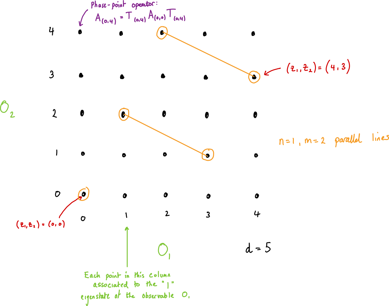
A graphical depiction of the phase space for the discrete Wigner function.
The Discrete Wigner Function:
Let . Given condition 2 stated above in the list of properties of phase-point operators, the set of phase-point operators form a complete basis for the set of Hermitian matrices. The discrete Wigner function, denoted at the point for the state , is then defined as
such that
The discrete Wigner function then satisfies the following properties
.
Let have Wigner functions and respectively, then
The phase space can be foliated into a set of parallel lines. For each line, given by , the sum over the Wigner functions for the points in , , describes the probability of a measurement associated to that foliation. The eigenstate associated to this measurement is that of the projection operator, given in condition 3, for the given foliation.
Note, the Wigner function can be negative, meaning it cannot be directly interpreted as a probability distribution. As with the state vector or density operator, it is instead an object from which probabilities of measurement outcomes can be found.
There are different foliations of the phase space into sets of parallel lines. As given in condition 3 above, a measurement can be associated to each set of parallel lines. The eigenbasis of the measurements associated to each set have mutually unbiased basis.
Composite Systems
The above was all for systems that are -dimensional where is a prime number. System that have a non-prime dimension can be build up out of systems that do have prime dimensions, such as systems.
Firstly, one factorises into prime numbers: , such that is prime for all . To each a phase space can be associated, that is an array of points . The total phase space is taken to be the Cartesian product of these phase spaces. Given two sets and , the Cartesian product is
Therefore, a point in the total phase space of a composite system is given by an ordered tuple of points from the different subsystems,
Note, the different subsystems can be different dimensions.
In composite systems, lines becomes slices. Given a set of lines, one from each subsystem, a slice is the set of points from all subsystems that are contained in the set of lines.
Phase-point operators can be found for these composite systems by taking the tensor product of the phase-point operators for the different subsystems,
All the properties of phase-point operators given above still apply for the phase point operators of composite systems but with notion of a line replaced by a slice.
The Wigner function for composite systems is calculated in the same way as for non-composite systems.
Further Properties
Definitions
The follow definitions are used in the below properties of the discrete Winger functions.
Clifford operators, , are the set of unitaries that map the Heisenberg-Weyl operators to themselves up to a phase. Specifically, a unitary if and only if
The set of stabliser states is the convex combination of states that can be reached from by the Clifford operators,
See Veitch et al. (2012) and Veitch et al. (2014) for more details.
Discrete Hudson’s Theorem (prime dimensions): A pure state, , is a stabliser state, , if and only if it has positve Wigner representation
Clifford operators act as permutations of the phase-space
Although, only the symplectic permutations of phase space correspond to clifford operators.
As discussed above, the phase-point operators are a basis for all Hermitian matrices. Hence, the trace of any Hermitain matrix can be found by summing over it’s Wigner function for all point in phase space,
where the fact that has been used.
Phase Space for General Hermitian Operators, POVMs and Channel
See Wang et al. (2019) more full details on these definitions.
General Hermitian Operators
Let be a Hermitian operator, such that .
The discrete Winger function at a point of the operator is given by
POVMS
Let be a POVM, so that and .
The discrete Winger function at a point of an operator is given by
where
Channels
Let be a quantum channel.
The discrete Winger function at a point of the operator is given by
where is the Choi-state of and is the phase point operator in the space at the point . It is the case that
Further Reading
For Wigner Functions in Discrete Spaces - A Wigner-function formulation of finite-state quantum mechanics
Review Article on quantum mechanics in phase space - Overview of the Phase Space Formulation of Quantum Mechanics with Application to Quantum Technologies
Review Article on general quasi-probability representations of quantum theory - Quasi-probability representations of quantum theory with applications to quantum information science
- Rundle, R. P., & Everitt, M. J. (2021). Overview of the Phase Space Formulation of Quantum Mechanics with Application to Quantum Technologies. Advanced Quantum Technologies, 4(6). 10.1002/qute.202100016
- Wootters, W. K. (1987). A Wigner-function formulation of finite-state quantum mechanics. Annals of Physics, 176(1), 1–21. 10.1016/0003-4916(87)90176-x
- Veitch, V., Ferrie, C., Gross, D., & Emerson, J. (2012). Negative quasi-probability as a resource for quantum computation. New Journal of Physics, 14(11), 113011. 10.1088/1367-2630/14/11/113011
- Veitch, V., Hamed Mousavian, S. A., Gottesman, D., & Emerson, J. (2014). The resource theory of stabilizer quantum computation. New Journal of Physics, 16(1), 013009. 10.1088/1367-2630/16/1/013009
- Wang, X., Wilde, M. M., & Su, Y. (2019). Quantifying the magic of quantum channels. New Journal of Physics, 21(10), 103002. 10.1088/1367-2630/ab451d
- Ferrie, C. (2011). Quasi-probability representations of quantum theory with applications to quantum information science. Reports on Progress in Physics, 74(11), 116001. 10.1088/0034-4885/74/11/116001